Understanding cloud droplet formation is fundamental in cloud physics. Water vapor condenses in the atmosphere on tiny aerosol particles when supersaturation slightly exceeds the equilibrium saturation. Köhler theory explains the equilibrium saturation of a solution droplet, such as a wetted aerosol particle, and thus determines whether it grows by condensation or shrinks by evaporation. If the ambient supersaturation exceeds its critical value, the particle grows freely, a process referred to as activation. The aerosol particle is considered a cloud droplet once it is activated. For a given ambient supersaturation, whether an aerosol particle of a given size and chemical composition is activated depends on its critical supersaturation. The activation spectrum describes the relationship between the number of activated particles and supersaturation. The activation spectrum, typically denoted as N(S) or NCCN(S) , is a cumulative distribution function. It describes the total number concentration of aerosol particles per unit volume of air that will activate and grow into cloud droplets at or below a specific environmental supersaturation, S. The exercise consists of calculating the activation spectrum for a given, constant supersaturation and comparing that result with the activation spectrum generated by a simple cloud model. In your exercise, you will be using a bimodal lognormal size distribution of dry aerosol particles. To get the activation spectrum from this, you must link the physical size of the dry particle (rd) to its critical supersaturation (Sc). Using Köhler theory, you determine the critical supersaturation Sc required to activate a particle of a given dry radius rd and chemical composition (often parameterized by the hygroscopicity parameter, κ). If the ambient supersaturation is S, any particle with a critical supersaturation Sc≤S will activate. This corresponds to all particles with a dry radius greater than some critical activation radius, rcrit(S). The activation spectrum is calculated by integrating the dry aerosol size distribution n(rd) from that critical radius up to infinity: 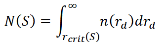
This physically derived spectrum shows that as ambient supersaturation increases, smaller and smaller particles (which are usually vastly more numerous) are forced to activate, causing N(S) to rise steeply. Bimodal lognormal aerosol size distributions parameters to be used in the exercise: Aerosol type | N1 (cm-3) | rd1 | σ1 | N2 (cm-3) | rd2 | σ2 | VOCALS | 60 | 0.020 | 1.4 | 40 | 0.075 | 1.60 | marine | 125 | 0.011 | 1.2 | 65 | 0.060 | 1.70 | polluted | 160 | 0.029 | 1.36 | 380 | 0.071 | 1.57 |
|
| Lab |
Numerical cloud models produce output in the form of 3-dimensional arrays of variables of interest (e.g., cloud water content). Visualizing this data, which helps in understanding model behavior and is useful for science outreach, is a separate task. In this lab, students will produce a video of a cumulus congestus cloud modeled with the UWLCM model (model output will be provided). The video will be made using ParaView — a standard tool for scientific visualization. ParaView can be used through Python. Python scripts that can be used as a starting point for this laboratory can be found here: https://github.com/igfuw/UWLCM_plotting/tree/master/paraview_scripts Example of a visualization from a different model: https://www.youtube.com/watch?v=dxoIdczz-gc |
| Lab |
UWLCM is a tool for numerical modeling of clouds using the Large-Eddy Simulation (LES) approach and detailed Lagrangian microphysics. Detailed cloud simulations are too costly to be run on a single computer. Instead, such simulations are performed on clusters of computing nodes with distributed memory (supercomputers). Communication between nodes incurs an additional cost that slows down such simulations. Therefore, to find an optimal balance between computation time and the usage of computational resources, it is necessary to perform scalability tests of the model, in which computational time is compared for a varying number of nodes. Various scenarios are considered, such as weak scaling (in which the problem size increases with the number of nodes) and strong scaling (in which the total problem size remains constant). An additional consideration for UWLCM is that it uses both CPUs and GPUs for computations, and the percentage of time both processing units work simultaneously depends on the number of nodes. Scalability tests on the Cyfronet Prometheus cluster are described in: https://gmd.copernicus.org/articles/15/4489/2022/ . The student's task will be to perform similar tests on a newer cluster. This may require setting up the environment to run the UWLCM model and finding optimal run parameters. Availability of this laboratory is subject to access to supercomputers. |
| Lab |
Turbulence kinetic energy dissipation rate (EDR) is the rate is an important parameter, used in parametrizations of atmospheric turbulence. It describes how the kinetic energy is converted into heat at the smallest scales. Due to finite frequency of instruments, these scales are typically too small to be measured in atmospheric turbulence. Hence, the turbulence kinetic energy dissipation rate is estimated using indirect methods. They assume that the rate at which the energy is injected into the system via production mechanisms is equal to the rate at which it is transfreed towards smaller scales and equal to the rate at which it is dissipated (converted into the internal energy) by the smallest eddies. The constant transfer rate in the intermediate range of scales results in the universal -5/3 scaling of the energy spectra (so-called Kolmogorov scaling). In this exercise, the indirect, iterative method proposed in Wacławczyk et al. (Atmos. Measur. Tech., 10, 2017) will be used for EDR estimates. The iterative method has several advantages over standard spectral estimates. In spectral methods a fitting range in which Kolmogorov scaling holds must be defined a priori. In contrast, the iterative method requires only the calculation of the time derivative of the time series, its standard deviation, and a correcting factor that accounts for the shape of the unresolved part of the spectrum. In this exercise a student will develop a python code which reads measurement data of wind velocity from MOSAiC database and estimates EDR using the iterative method. |
| Lab |
A stable atmospheric boundary layer (SBL) forms when the air near the surface is colder than the air above,
creating a temperature inversion that suppresses vertical motion. SBL is typically observed during clear nigths over land
or over cold surfaces like ice in the Arctic. The vertical mixing in SBL is suppressed by the negative
buoyancy. Turbulence is driven by wind shear and often becomes intermittent and patchy.
In this task MOSAiC database from Arctic will be used to perform Reynolds decomposition of wind and temperature into the
mean and fluctuating part. For this, different sizes of averaging windows will be used to investigate how they affect
the decomposition. Next, Reynolds stresses and heat fluxes will be calculated and stability of the surface layer will be
estimated. |
| Lab |
This exercise is an introduction to computer simulations using particles. The method of smoothed particle hydrodynamics (SPH) will be used to study some nonlinear phenomena of relevance for atmospheric physics. Programing skills and basic knowledge of theoretical methods in hydrodynamics are required for this task. |
| Lab |
Large Eddy Simulation (LES) technique has become an important tool in the atmospheric turbulence research.
In this method the largest eddy structures are resolved on a numerical grid, while the effect of smaller
(subgrid) eddies is taken into account through a proper closure. John Hopkins Turbulence Database contains
datasets with results of Direct Numerical Simulations and Large Eddy Simulations of various test
cases, including geophysical rotating stratified turbulence and LES of the stably stratified atmospheric boundary layer.

Within this task a student will get acquainted with the basic data formats used to store the data and learn
about methods to download and post-process the data. The task is to calculate mean quantities like mean velocity,
mean temperature and fluxes from the given fields and plot them as a function of height. The student
will calculate the Obukhov length and study turbulence statistics in the region of the surface layer,
as well as identify the presence of the Ekman spiral at larger altitudes. |
| Lab |
In this exercise, a student will investigate how horizontal temperature differences in a rotating fluid generate vertical variations in velocity, a phenomenon known as thermal wind balance. This is a fundamental concept in geophysical fluid dynamics, which helps explain large-scale phenomena such as jet streams and ocean currents. In this task a cylindrical tank filled with water will be placed on a rotating table. Cubes of ice will be placed at the center of the tank to create a localized cold region. Next, the system will be set into steady rotation and allowed to reach solid-body rotation. A student will inject dye at different depths and positions around the ice cube and observe and sketch the flow pattern at different depths. They will identify how the presence of the cold core (ice) affects the velocity structure of the fluid, discuss how the temperature difference created by the ice cubes influences the pressure field and how this is related to the balance between pressure gradients and the Coriolis effect. The important outcome will be to identify in what way is this experiment analogous to atmospheric or oceanic flows. |
| Lab |
| Class |
The aim of the exercise is to derive the profiles of the aerosol depolarization (UV and VIS), water vapour mixing ratio, and fluorescence efficiency from the European Space Agency Mobile Aerosol Raman EMORAL lidar signals. Student will use lidar measurements for different cases, e.g. Rayleigh atmosphere, air-mass of biomass combustion, and air mass of mineral dust. She/He will write numerical programs or use an existing software for the retrieval of the aforementioned profiles in the atmosphere, estimate the measurement uncertainties, and perform a comparative analysis of the diffrent cases. The feasibility of using the obtained information for aerosol typing will be assessed. |
| Lab |
The aim of the exercise is Langley calibration of the Multifilter Rotating Shadowband Radiometer and deriving aerosol optical depth and Angstrom exponent. Student will work with data from MFR-7 mounted in Radiative Transfer Laboratory at the roof platfor of the Institute of Geophysics. During the exercise, the data processing will be done, including several corrections. |
| Lab |
The aim of the exercise is to analyse properties of biomass-burning aerosol. The goal is to derive profiles of aerosol optical properties, depolarization ratio and relative humidity, so as to characterize the atmosphere using the signals of ADR-PollyXT lidar and NARLa lidar. The student will use available lidar observations in combination with weather profiling of radiosounding and photometric measurements. The data will be processed using available numerical programs, including estimates of measurement errors. For the analysis and interpretation of the processed data, the student will use the methodology proposed by him/herself. |
| Lab |
The exercise aims at determining effects of relative humidity on optical and microphysical properties of aerosol in laboratory conditions. Measurements will be conducted using the aerosol condition system (ACS1000), which allows for applying controlled changes of relative humidity upon the air collceted using the inlet located on the measuring platform. The chamber consists of two measuring paths: one that contains dehumidified air with low relative humidity (approx. < 30%), while the other contains air that moves through a special moisturizing system enabling the setting of desired humidity value in the range from 40 to 90%. Both measurements take place simultaneously with the used of miniature OPC-N3 particle counters. This enables to determine changes in the particle size distribution and the scattering coefficient as the air humidity changes. |
| Lab |
Mixed-phase clouds are three-phase systems consisting of water vapor, ice particles and supercooled liquid droplets. In this exercise the student will model and simulate the phase partitioning of water condensate in mixed-phase clouds using a bulk microphysical approach. Simulations will be made for the adiabatic cloud parcel model. We plan the following course of the exercise: learning the model equations and the thermodynamics of mixed-phase systems, developing the numerical code and conducting calculations for various model parameters. The simple modeling approach used in this exercise should provide reference results for testing and development of more sophisticated microphysical schemes. |
| Lab |
Size distribution of droplets and their concentration in a unit volume are basic microphysical properties characterizing the cloud. Knowing both, one can also calculate total liquid water content. The goal of the exercise is to introduce the method of measuring those parameters with shadowgraphy. Student’s tasks include the lab measurement of droplet sizes and concentrations in the streams generated by a few different devices (e.g. pond mist maker, household humidifier, flower sprayer, nasal hygiene spray), comparing the properties of the obtained size distributions and estimating total liquid water content. For ambitious: The second goal of the exercise is to introduce optical techniques for measuring size distribution and fall velocity of rain drops, as well as rainfall rate. Student task’s involve selecting the proper experiment time based on weather forecast, measuring rain drop sizes and velocities at the roof of the institute building with shadowgraphy technique and comparing the results with routine observations performed with a disdrometer. | | Lecture documents: |
Measurement of cloud droplet size and concentration with shadowgraphy - instructions -
Script for the classes
shadowgraph_intro_JN2020.pdf |
| Lab |
Goal of this exercise was to characterize properties of atmospheric aerosols over three different sites. For this purpose the AERONET sun photometer database will be used. The measurement sites will be chosen by the student and reasoning for the choice need to be carefully explained. The data for at least one year at each site need to be investigated. For the daily average values of aerosol optical depth and Angstrom exponent a classification into 3 groups with low, medium and large values need to be done, followed by description of each. This topic can be realized in extended version with use of the ocean color data and lunar data. |
| Lab |
The aim of the exercise is to derive properties of minerat dust agigination if African or Asian deserts. The profiles of aerosol optical properties, depolarization ratio and relative humidity will be obtained, so as to characterize the atmosphere using the signals of ADR-PollyXT lidar and NARLa lidar. The student will use available lidar observations in combination with weather profiling of radiosounding and photometric measurements. The data will be processed using available numerical programs, including estimates of measurement errors. For the analysis and interpretation of the processed data, the student will use the methodology proposed by him/herself. |
| Lab |
Student will analyse the data collected during measurement campaign involving scanning lidar observations of aerosphere and ocean over the Tresna lake in Poland. The observations were conducted in October 2024 using the scanning lidar of University of Silesia. Assessment of the scanning lidar data at four channels (2 aerosol, water, nitrogen) at different incidence angles into the water surface will be done. Analysis aims at determining the penetration depth and optical depth investigations. |
| Lab |
Turbulent Kinetic Energy (TKE) dissipation rate is a key physical quantity characterizing turbulent air motions present in the atmosphere. According to Kolmogorov’s theory, its value can be derived from velocity fluctuations, measured e.g. with a stationary ultrasonic anemometer or various airborne instruments. The goal of the exercise is to learn several approaches for estimation of TKE dissipation rate (power spectrum, structure functions, number of crossings), apply them for the velocity data collected routinely at the top of the institute building and compare the results for the period of a few days. |
| Lab |
Students will learn how to run and analyze numerical simulations of clouds. Simulations will be done using the University of Warsaw Lagrangian Cloud Model, a state-of-the-art model developed at IGF. Data analysis will make use of the Xarray Python package. Both simulations and data analysis will be done through a Jupyter Notebook ran on a supercomputing cluster. Basic knowledge of Python programming language is the only prerequisite for this laboratory. | | Lecture documents: |
Task description -
Script for the classes
Cloud_modeling_introduction.pdf
|
| Lab |
The ultrasonic anemometer installed ontop of the institute building records three components of the air flow velocity and virtual temperature at a rate up to 32 Hz. Measured fluctuations of velocity and virtual temperature allow for the calculation of turbulent fluxes of momentum and heat in the boundary layer of the atmosphere with the use of eddy correlation method. Relationship between those quantities determines, in turn, the dynamic stability in the layer, which is customarily expressed by the Monin-Obukhov length. Student’s tasks involve performing Reynolds decomposition of the recorded signals, calculating respective turbulent fluxes, deriving Monin-Obukhov length and analyzing its variability in the course of a few selected days. |
| Lab |
Rain drops are formed through coalescence of smaller droplets, which is a consequence of collisions between droplets. Student task will be to model the collision-coalescence process using a probabilistic description. The goal is to quantify the number of "lucky" droplets, which are droplets that undergo a series of unlikely collisions and grow to much larger sizes than average droplets. Results will be compared with theoretical estimates. This exercise is intended as a follow-up to the exercise "Simple model of collision-coalescence in clouds". |
| Lab |
The main goal of this study is to update a simple global mean, zero-dimensional, climate model developed by University of Reading and to run simulation to estimate the optimal model parameters. This two layer aqua planet model solve two differential equations for mixed layer and deep layer temperature anomaly which is forced by the mean radiative forcing. The main task is to extend the simulation to 2019 based on last IPCC data. The next one is to develop the minimization method to estimate the best model parameters based on observation data and model results. |
| Lab |
This exercise concerns the numerical calculation of scalar advection (temperature and water vapor) in a synthetic cloud flow. Condensation is performed using an instantaneous saturation adjustment scheme. This simple condensation model should provide reference results for testing and development of more sophisticated cloud microphysical schemes. Programming skills and basic knowledge of cloud physics are required. |
| Lab |
| Lab |
The rate of sublimation is commonly calculated using simple Hertz-Knudsen equation. This equation was derived ignoring microstructure of material and assuming equilibrium distribution of the velocities of molecules condensing on the surface and leaving it. Thus, is it gives only approximate result. It can be corrected using temperature dependent sublimation coefficient (e.g. Kossacki et al. 1999; Gundlach et al. 2011; Kossacki et al. 2017). Exercise: Sublimation of ice is investigated in laboratory, using cooled vacuum chamber. Measured parameters are: position of the surface and the temperature. Student is expected to perform measurement and derive the temperature dependent rate of sublimation. This exercise is dedicated to advanced student. Note that, due to the COVID-19 situation, the student will receive raw measurement data for analysis. |
| Lab |
In this excercise, a student will use a rotating table to demonstrate the formation of a Taylor column, a phenomenon arising from the Coriolis effect in a rotating fluid system. The tank filled with water will be set into steady rotation. A small obstacle (e.g., a cylinder) will be introduced on the bottom of the tank. After the fluid reaches solid-body rotation a student will inject dye upstream of the obstacle and observe how the flow behaves. The task includes: - Observing and sketching the flow pattern,
- Identifying conditions under which the Taylor column forms,
- Relating observations to rotating fluid dynamics concepts.
The goal is to understand how rotation influences fluid motion and suppresses vertical flow. |
| Lab |
The exercise is aimed at determination of the thermal conductivity of granular ice, or natural snow (if it is available) without sampling the test material. The measurement is made using linear probe technology. It is used in practice in situations when taking a sample of the material is inexpedient or technically impossible. This method is applied to investigate directly (in-situ) properties of cosmic bodies using automatic landing probes, e.g. comet Churyumov-Gerasimenko (mission Rosetta, experiment MUPUS). Idea is the following: changes of the temperature of a long thin heater inserted in a solid material is a function of its thermal conductivity. When the heating power is known it is sufficient to register changes of the temperature. The latter can be done automatically. Student is expected to perform 2 -3 measurements and analyze the source data. This exercize is dedicated to advanced student. Note that, due to the COVID-19 situation, the student will receive raw measurement data for analysis. |
| Lab |
The aim of this exercise is to study processes of formation and evolution of cloud droplets. It will be realized using an existing numerical parcel model (https://github.com/igfuw/parcel). Main tasks include: getting acquainted with the model documentation, installation of the model, running of a set of numerical simulations. Results obtained will have to be thoroughly analyzed in order to identify parameters having impact on droplet size distribution. Realization of this exercise will result in effective understanding of parcel model as a tool used in numerical simulations of cloud processes, and also deeper understanding of cloud microphysical processes. |
| Lab |
The exercise is aimed at determination of the thermal conductivity of sand without sampling the test material. The measurement is made by linear probe technology. It is used in practice in situations when taking a sample of the material is inexpedient or technically impossible. This method is applied to investigate directly (in-situ) properties of cosmic bodies using automatic landing probes, e.g. comet Churyumov-Gerasimenko (mission Rosetta, experiment MUPUS). Idea is the following: changes of the temperature of a long thin heater inserted in a solid material is a function of its thermal conductivity. When the heating power is known it is sufficient to register changes of the temperature. The latter can be done automatically. Student is expected to perform 2 -3 measurements and analyze the source data. Alternatively, student may process the existing source data. This exercise is dedicated for beginner student. |
| Lab |
The finite inertia of droplets in a turbulent fluid causes droplets to diverge from regions of high vorticity and to converge preferentially in regions of low vorticity. This creates strong deviations from uniformity in droplet concentration. The aim of the exercise is to simulate the motion of droplets (modeled as point-particles) in a synthetic turbulent flow under the influence of gravity. Simulation results should explain to what extent droplet inertia, gravity, and turbulence affect droplet spatial distribution. |
| Lab |
This exercise concerns the estimation of turbulence statistics from time series recorded by a fixed-point sensor. For such estimates, it is usually assumed that the wind velocity spectrum follows Kolmogorov scaling at small scales. To convert the measured time series into space-dependent data, the Taylor frozen-eddy hypothesis is typically employed, in which the mean wind velocity is assumed to advect turbulence structures past the sensor without distortion. This assumption works well for strong winds and when the turbulence intensity I (the ratio of the root-mean-square of wind velocity fluctuations to the mean wind speed) is small. However, the Taylor hypothesis is not always valid, for example, in the convective regime with weak winds. In this case, the sweeping of small eddies by larger ones becomes an important mechanism, significantly affecting the frequency spectra. In addition, the measured time series are subject to effective spectral cut-offs due to the finite sampling frequency of the sensor. In this exercise, the student will calculate turbulence statistics from time series of wind velocity recorded under convective conditions and evaluate how they are affected by random sweeping and finite sampling frequency. A correction accounting for these effects will then be applied. |
| Lab |
Doppler lidar system allows for obtaining vertical profiles of wind vector within the atmospheric boundary layer with high spatial and temporal resolution for atmospheric applications. The aim of this exercise is to be able to filter and process the data to properly represent, understand and interpret different patterns observed with Doppler lidar (e.g. related to nocturnal jets or daytime convection). The analysis will cover several examples measured over a peatland site in Rzecin and/or at urban site in Warsaw. |
| Lab |
The aim of the exercise is to retrieve the aerosol size distribution on the basis of spectral aerosol optical depth measurements by hand-held MICROTOPS sun photometer. The aerosol size distribution will be approximated by two log-normal distributions based on minimizing the cost function. During minimization, 2 or 4 parameters describing the size distribution are determined. The data can be obtained by the student her/him-self using one of our MICROTOPS instruments. Alternatively, student can use the already permormed observations from diferent field campaigns in Poland (Sopot, Kraków, Wrocław) and abraod (Vilnius, Orasac-Dubrovnik, Athens, Magurele-Bucharest, Ny-Alesund). |
| Lab |
The aim of the exercise is to estimate the aerosol radiation forcing on the basis of observation of surface solar flux and radiative transfer simulation of aerosol-free solar fluxes. In addition, the radiation budget at Earth’s surface will be determined, as well as the total energy budget, including sensible and latent heat fluxes. |
| Lab |